Table of Links

Abstract and 1. Introduction

2. Methods

2.1. Modeling Panspermia and Terraformation

2.2. Identifying the Presence of Terraformed Planets and 2.3. Software and Availability

3. Results

3.1. Panspermia can increase the correlation between planets’ compositions and positions

3.2. Likely terraformed planets can be identified from clustering

4. Summary and Discussion

5. Acknowledgements and References

APPENDIX

A. Appendix

2.2. Identifying the Presence of Terraformed Planets

2.2.1. Summary

We hypothesize that the process of panspermia and terraformation in our model will lead to a population of planets with anomalously high positive correlations between their spatial locations and compositions, compared to random permutations of these planets’ compositions. We quantify this using the Mantel test—a statistical test common in ecological science (Sec. 2.2.2). By clustering on the planet compositions, we can begin to pin down clusters of planets driving these correlations (Sec. 2.2.3). From these initial clusters, we select those localized in space (via their interquartile range, IQR), because we hypothesize that life would not only change the distribution of planetary compositions, but would also do so in a relatively compact portion of the galaxy. We further select clusters which, when removed, cause a decrease in the Mantel coefficient of the residual space of planets (Sec. 2.2.4). Finally, we attempt to evaluate how well our clusters reflect the presence of truly terraformed planets (Sec. 2.2.5).

2.2.2. Mantel Test

The Mantel test is a measure of correlation between two distance matrices. The resulting value is called the Mantel coefficient, and is reported alongside a p-value calculated from an approximate permutation test (indicating the proportion of randomly permuted distance matrices which have correlations greater or equal to the correlation between the non-permuted distance matrices). Simply put, the p-value indicates how unlikely this correlation is compared to random permutations of the data. We wrote the Mantel test in Julia, with the algorithm and code adapted from Python’s scikit-bio (The scikit-bio development team 2020; Rideout et al. 2023). Here we used the Mantel test to measure the Pearson correlation between a distance matrix of all planet positions, and a distance matrix of all planet compositions. For each Mantel coefficient calculation, the p-value was generated using 99 permutations with a 2-sided alternative hypothesis. This is approximately equal to 2.5σ confidence. Because the p-value quantifies how anomalous an observed composition/position association is, given the assumptions of the model that correlations should only occur from panspermia and terraformation, we treat the p-value as one measure of confidence in the space containing a biosignature. To get an idea of how sensitive the Mantel coefficient corresponding to a 2.5σ detection is, we plotted how it varies based on number of planets observed (Fig. A3). We find that the sensitivity of the Mantel coefficient to number of planets observed decreases exponentially, and 1000 planets seems like a reasonable choice to reflect the balance of the challenge of realistically observing planets, with the need for those planets to exhibit potentially small correlations in composition-position space. The exact shape of this plot will vary by model parameters, but is especially dependent on the distribution of planet compositions and positions (e.g., planets being evenly distributed in composition or position space, vs. extremely heterogeneous).

2.2.3. Clustering

We clustered planets in each iteration of the simulation based only on their compositions, using the DBSCAN algorithm implemented in R (Hahsler et al. 2019). Briefly, compared to other clustering algorithms, DBSCAN does not require the number of clusters to be predefined, can identify clusters of varying shapes and sizes based on the density of data points in the feature space, and separates points as belonging to clusters or noise. Arguments were chosen based on advice in the documentation, with minPts = 11 (the dimensionality of the data + 1), and eps was chosen dynamically at each iteration based on the location of the elbow in the k-nearest neighbor distance plot. Because the location of the elbow is not always obvious, we used the R implementation of the Kneedle algorithm (Satopaa et al. 2011), with sensitivity parameter = 1, empirically determined based on visual examination of the elbow placement on the nearest neighbor curves (Fig. A4). Note that the sensitivity should be adjusted to the specific data being analyzed, and in our case the data changes at each time step. This results in the Kneedle sensitivity being appropriate for only part of the time steps in our simulation. We chose to focus on the early steps of the simulation, but the sensitivity should be adjusted if finding the curves’ elbows in later time steps. DBSCAN classifies each point (planet) as either being part of a particular cluster, or noise (meaning it does not meet the criteria to fall into a cluster based on our chosen arguments).

2.2.4. Selecting clusters

We first sought to select clusters for their likelihood of containing terraformed planets, without the aid of ground truth labels (i.e., without using our knowledge of which planets were truly terraformed in the model). We selected them by measuring their spatial spread, and by analyzing how the Mantel coefficient of the residual space of planets changes when removing clusters of planets.

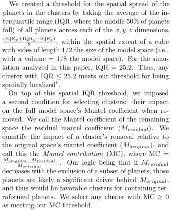
We created a threshold for the spatial spread of the planets in the clusters by taking the average of the interquartile range (IQR, where the middle 50% of planets fall) of all planets across each of the x, y, z dimensions,

2.2.5. Evaluating clustering

We evaluated selected clusters meeting our criteria (IQR ≤ 25.2 ∧ MC ≥ 0) for how well they identified terraformed/non-terraformed planets, based on the true labels of each planet throughout our simulation.

At each iteration, for each selected cluster, we calculated the ratio of planets in the cluster which were terraformed (true positives, TP) and non-terraformed (false positives, FP), as well as the ratio of planets outside the cluster which were non-terraformed (true negatives, TN) and terraformed (false negatives, FN) (Fig. A13). For example, if 100 of 1000 planets are terraformed, and a single selected cluster is identified with 80 planets, only 75 of which are terraformed, then the ratios for each metric in this cluster are: TP = 75/80, FP = 5/80, TN = 895/920, FN = 25/920.

To simplify how this information is conveyed, we report the summary statistics of sensitivity, specificity, and accuracy.

• Sensitivity is the proportion of all terraformed planets correctly selected by the cluster, TP/(TP+FN). This is 75/(75 + 25) in our example.

• Specificity is the proportion of all non-terraformed planets correctly not selected by the cluster, TN/(TN+FP). This is 895/(895 + 5) in our example.

• Accuracy is the proportion of all planets correctly classified, TP+TN/(TP+FP+TN+FN). This is (75 + 895)/1000 in our example.

We believe a reliable biosignature must minimize false positives (i.e., must not misclassify non-terraformed planets), even at the expense of producing false negatives (i.e., missing terraformed planets). We thus consider our evaluation to be successful in validating our approach if specificity is high, even if sensitivity is low.

2.3. Software and Availability

The code necessary to run the simulations and analyses is available on Github at https://github.com/ hbsmith/SmithSinapayen2024. Simulations were built in Julia, and analyses were carried out in Julia, Python, and R.

This paper is available on arxiv under CC BY-NC-ND 4.0 Deed license.

[6] Though the extent we chose for an IQR threshold is arbitrary, it reflects the relative size of our model space and the presumption that looking for life that is still relatively spatially localized is of greater interest than looking for life which has already spread over the galaxy (the latter implying there might be other easier ways to look for life). This choice, like others, could be modified depending on other assumptions or objectives.