A Biosignature Based on Modeling Panspermia and Terraformation: Appendix
2024-8-17 03:0:17 Author: hackernoon.com(查看原文) 阅读量:8 收藏

Abstract and 1. Introduction

2. Methods

2.1. Modeling Panspermia and Terraformation

2.2. Identifying the Presence of Terraformed Planets and 2.3. Software and Availability

3. Results

3.1. Panspermia can increase the correlation between planets’ compositions and positions

3.2. Likely terraformed planets can be identified from clustering

4. Summary and Discussion

5. Acknowledgements and References

APPENDIX

A. Appendix

APPENDIX

A. APPENDIX

A.1. The mantel coefficient does not strictly increase with the proliferation of life

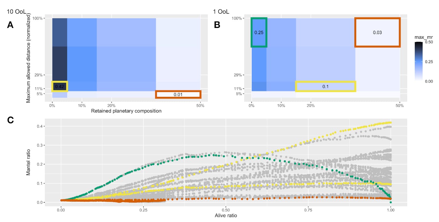
We investigated how changing the parameters of our model influenced the Mantel coefficient as a function of the ratio of terraformed planets. We find a few characteristic shapes of curves observed: flat, increasing then decreasing, and mostly increasing.

A.1.1. Additional Parameters

Mutation. Depending on the scenario, we include either a 0% or 10% chance of mutation for each element of the planet’s new composition, meaning that in the 10% scenario, with our length 10 composition vector, on average, 1 of the 10 elements is mutated during each terraformation event. Mutated elements are chosen from a continuous uniform random distribution of [0, 1], just like the initial compositions were chosen. Mutation is meant to represent the change in the kind of planetary observable characteristics which are compatible with life as life evolves over time.

Number of origins of life (OoL). Simulations are initialized with either 1 or 10 OoL (Fig. A2).

Compositions inherited from pre-terraformed planet. We vary the number of elements that the post-terraformed planet inherits from the pre-terraformed planet, n ∈ [0, 1, 2, 5], with the rest of the composition inherited from the incoming life.
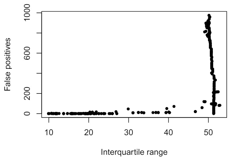
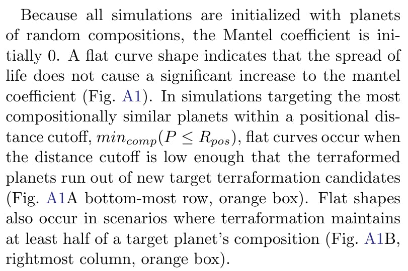
A.1.2. Flat curve

A.1.3. Increasing then decreasing curve

When simulations are initialized with a single OoL, the progression of planet terraformation over time leads to an increasing then decreasing shaped Mantel coefficient curve, where the Mantel coefficient peaks after some of the planets have been terraformed, and then decreases afterwards (Fig. A1, data in green). Because the Mantel coefficient is measuring the correlation between positional and compositional distance matrices of planets, this correlation will decrease if either distance matrix becomes too homogeneous. With a single OoL, this is exactly what begins to happen with the compositional distance matrix, with the decline especially pronounced in the scenario with perfect replication (Fig. A1B, green box).

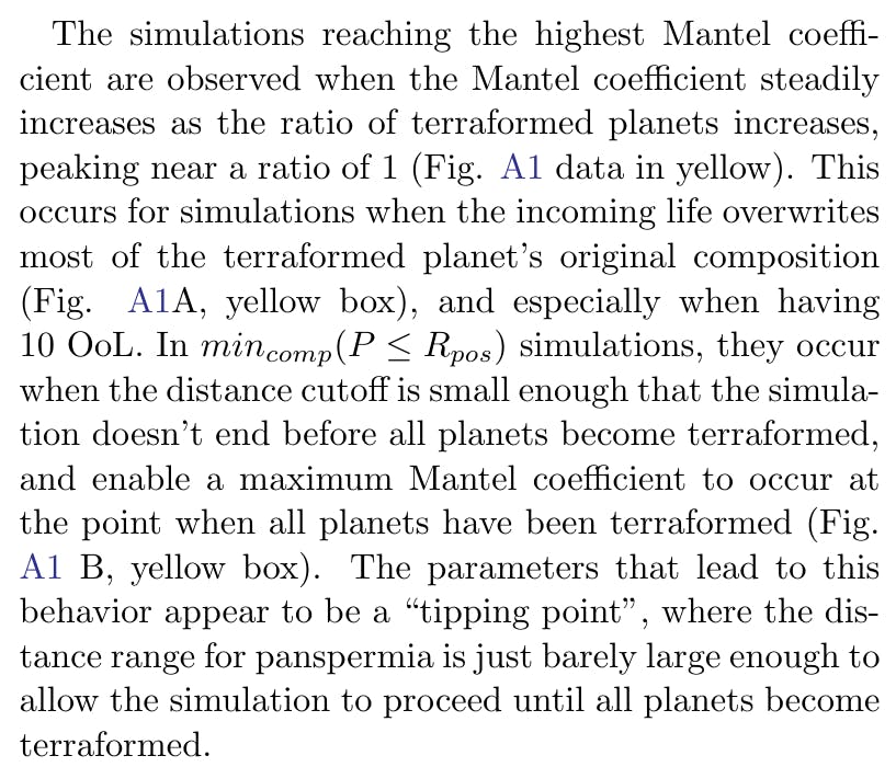
A.1.4. Mostly increasing curve

Figure A1. The impact of model parameter changes on the Mantel coefficient. Examples corresponding to “flat” (orange), “increasing than decreasing” (green), and “mostly increasing” (yellow). A and B show heatmaps for the maximum Mantel coefficient reached when varying the the amount of planetary composition retained by the terraformed planet after terraformation (x-axis), and varying the maximum allowed distance for planet target selection (y-axis), for scenarios with 1 OoL (A), and 10 OoL (B). C. The Mantel coefficient across different scenarios as a function of the terraformed planet ratio (x-axis).

Figure A2. Effect of complete terraformation, dependent on number of OoL. Simulations are initialized with either 1 or 10 origins of life, leading to different dynamics of compositional evolution.

Figure A3. A sensitivity analysis of the Mantel coefficient corresponding to a 2.5σ and 5σ anomaly, as a function of the number of planets observed. Positions and compositions of planets are chosen as in our model (See Methods Sec. 2) We find that the sensitivity of the Mantel coefficient to number of planets decreases exponentially, and 1000 planets seems like a reasonable choice to reflect the balance of the challenge of realistically observing planets, with the need for those planets to exhibit potentially small correlations in composition-position space. The exact shape of this plot will vary by model parameters, but is especially dependent on the distribution of planet compositions and positions (e.g., planets being evenly distributed in composition or position space, vs. extremely heterogeneous; not shown)

Figure A4. Elbow detection using the Kneedle algorithm for t=105 (left) and t = 205 (right) with different values of the sensitivity parameter. The elbow value has a huge influence on the quality of clustering. The curves on the right can be argued to have 3 elbows; 1 steep convex elbow, 1 soft convex elbow, and 1 concave elbow. We are interested in the steepest convex elbow, and therefore choose a sensitivity = 1 in this paper.

Figure A5. Mantel coefficient of each of the clusters as a function of the ratio of terraformed planets in the whole space. In grey are the clusters labeled as “noise” by the DBSCAN algorithm. The vertical dashed line represents the earliest detection of a cluster of terraformed planets using our proposed approach. The solid curve is the Mantel of the total space.

Figure A6. P-value of the Mantel coefficient of each of the clusters as a function of the ratio of terraformed planets in the whole space. In grey are the clusters labeled as “noise” bythe DBSCAN algorithm. The vertical dashed line represents the earliest detection of a cluster of terraformed planets using our proposed approach. The solid curve is the p-value of the Mantel coefficient of the total space.

Figure A7. Number of false positives in each cluster as a function of the cluster’s own Mantel coefficient. While the curve has a fascinating shape, we can see that there is no easy correlation.

Figure A8. Number of false positives in each cluster as a function of the cluster’s p-value for its Mantel coefficient. We can see that there is no simple correlation.

Figure A9. Number of false positives in each cluster as a function of the cluster’s IQR.

Figure A10. Number of false positives in each cluster as a function of the MC. There is a clear divide between the negative and positive MC.

Figure A11. Number of false positives in each cluster as a function of the residual Mantel coefficient. We can see that there is no simple correlation.

Figure A12. Number of false positives in each cluster as a function of the residual p-value. We can see that there is no simple correlation.

Figure A13. Ratios of true positives, false positives, true negatives and false negatives when changing the MC threshold in our selection critera. These results are for clusters below our IQR threshold of 25.2.

Authors:

(1) Harrison B. Smith, Earth-Life Science Institute, Tokyo Institute of Technology, Ookayama, Meguro-ku, Tokyo, Japan, and Blue Marble Space Institute of Science, Seattle, Washington, USA ([email protected]);

(2) Lana Sinapayen, Sony Computer Science Laboratories, Kyoto, Japan and National Institute for Basic Biology, Okazaki, Japan ([email protected]).


This paper is available on arxiv under CC BY-NC-ND 4.0 Deed license.


文章来源: https://hackernoon.com/a-biosignature-based-on-modeling-panspermia-and-terraformation-appendix?source=rss
如有侵权请联系:admin#unsafe.sh