Table of Links

Abstract and 1. Introduction

2 Model and 2.1 Optimal Stopping and Obstacle Problem

2.2 Mean Field Games with Optimal Stopping

2.3 Pure Strategy Equilibrium for OSMFG

2.4 Mixed Strategy Equilibrium for OSMFG

3 Algorithm Construction and 3.1 Fictitious Play

3.2 Convergence of Fictitious Play to Mixed Strategy Equilibrium

3.3 Algorithm Based on Fictitious Play

3.4 Numerical Analysis

4 Numerical Experiments and 4.1 A Non-local OSMFG Example

4.2 A Local OSMFG Example

5 Conclusion, Acknowledgement, and References

3.3 Algorithm Based on Fictitious Play

Theorem 3.1 provides the convergence result of the fictitious play as in Definition 3.1. We can turn the fictitious play into the following algorithm for finding the mixed strategy equilibrium.

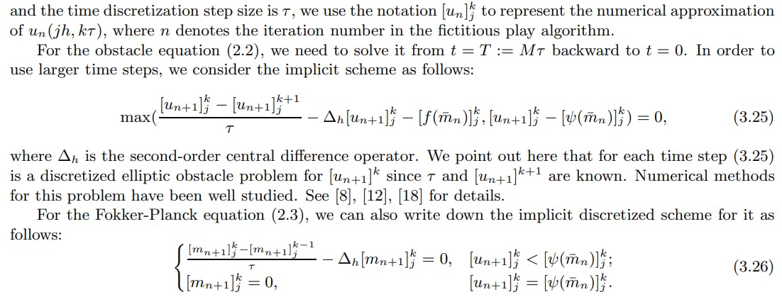
In the remainder of this section, we will introduce the discretization method for the obstacle equation (2.2) and the Fokker-Planck equation (2.3) in algorithm 1. Assuming the spatial discretization grid size is h

However, iteration are unavoidable when numerically solving equations (3.25) and (3.26), regardless of the method used. The application of nonlinear solvers renders the implicit scheme computationally inefficient. Therefore, in practice, semi-implicit schemes are preferred to reduce the computational cost. The semi-implicit scheme for u can be written as follows:

And the semi-implicit scheme for m can be written as:

Semi-implicit schemes for u and m can be viewed as a two-step method that decouples the linear and nonlinear parts of each equation. In the first step, u and m are evolved using a standard implicit scheme on the whole domain. In the second step, a cutoff is applied to u and m respectively to account for the free boundary effects. We only need to solve a sparse system of linear equations for each time step in the semi-implicit schemes (3.27) and (3.28.

Now we can summarize the finite difference algorithm into the following algorithm.