2024-10-18 07:11:54 Author: hackernoon.com(查看原文) 阅读量:1 收藏
The field of artificial intelligence is booming; image generation is one of the most prominent domains. There are a lot of competitors on the market, such as Stable Diffusion, Midjourney, and DALL-E. All these products are based on the diffusion networks approach. Unlike GPT diffusion models often seen as abstruse, the goal of this story is to demystify the complexity of diffusion models and explain how they work in an easy but comprehensive way. Let’s go!
The Basics
The Diffusion networks are artificial neural networks that allow you to solve various generation tasks. The most well-known application is image generation. In this story, let’s focus just on this type of generation. There are countless flavors of generation tasks: image2image, image2video, text2vide, video+image2video, etc. But all of them are based on a similar structure.
The diffusion network is composed of 3 building blocks (neural networks):
- Diffusion process: a process of image generation;
- Conditioning: a way to restrict generation to a given subject;
- Latent space: a trick that makes the model feasible to run in given hardware constraints.
Diffusion Process
The diffusion processes concept comes from physics, which describes the way particles spread in a medium over time. In the context of machine learning, a diffusion model learns to progressively "refine" a noise vector into meaningful data by reversing a diffusion-like process training set created from images by gradually adding more and more noise to each image.

To sample/generate from this model, we apply the network multiple times to minimize the noise and recover the image (denoising). Different diffusion models use different numbers of steps and different approaches for generating noise.
Conditioning
Conditioning introduces a dependency on additional information (text prompts in our case). This will allow us to generate samples that meet specific constraints.
-
We have to convert the text prompt to embedding to capture the semantics of our prompt (“e.g.: astronaut riding bicycle”).
-
We train denoising to adhere more closely to the textual semantics of our semantics.
Latent Space
The last building block is latent space. Typically, generative models operate in pixel space. However, inference in pixel space is expensive, and pixel space is sparse. The solution is to compress our initial image into a more compact representation, which exhibits better scaling properties with respect to the spatial dimensionality.

This compression is achieved using VAE (variational autoencoder models). This type of encoding differs from “vanilla“ autoencoders; it encodes images to a distribution with permitters μ and σ. This approach allows the introduction of generative properties for latent space. I will not explain the details here. Check out this post for more details.
The diffusion process is conducted in latent space.
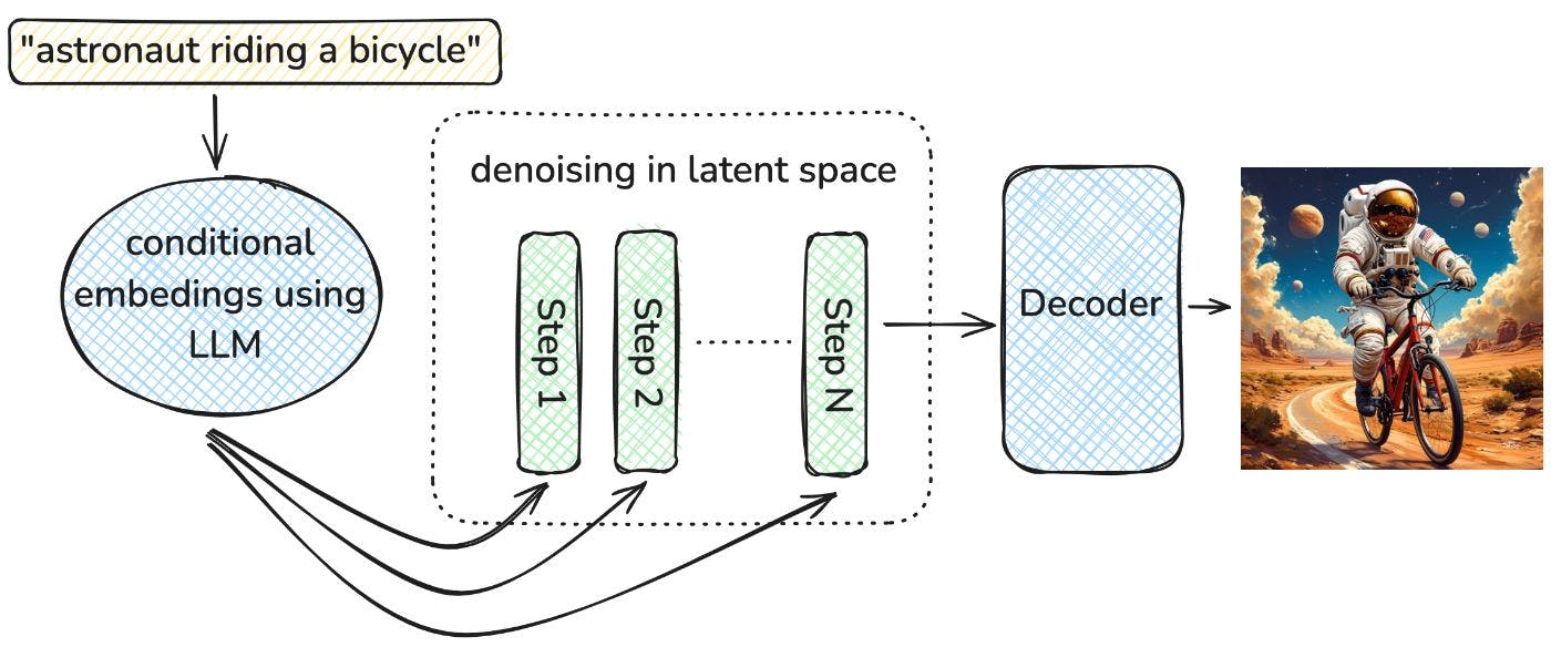
Putting Everything Together
Now, we studied all key components. It’s time to put everything together.

The whole process step-by-step:
- We get our prompt “astronaut riding bicycle.“
- The prompt is compressed to embedding representation; this representation will condition generation.
- The denoising process is performed in latent space with respect to the condition.
- The last step state in latent space is decoded to pixel space.
- We finally got our picture!
Links/Papers to Read
- High-Resolution Image Synthesis with Latent Diffusion Models: https://arxiv.org/abs/2112.10752
- Auto-Encoding Variational Bayes: https://arxiv.org/abs/1312.6114
- Reproducing Stable Diffusion from scratch, easy to read GitHub repo https://github.com/juraam/stable-diffusion-from-scratch
如有侵权请联系:admin#unsafe.sh