Table of Links

Abstract and 1 Introduction

2 Related Work

3 Framework

4 Main Results

5 A Case Study on Shortest-Path Distance

6 Conclusion and Discussion, and References

7 Proof of Theorem 1

8 Proof of Theorem 2

9 Procedure for Solving Eq. (6)

10 Additional Experiments Details and Results

11 Other Potential Applications

5 A Case Study on Shortest-Path Distance

In this section, we present a case study which utilizes the shortest path distance to validate the predictions and effectiveness of our proposed framework. We aim to demonstrate how our framework can be applied to a real-world scenario and how it can be used to understand the generalization performance of GNNs on different structural subgroups. The case study will provide insights and show the potential impact of our results on various critical applications of GNNs. In this case study, we aim to answer empirically the following questions: Given a GNN model that can preserve certain structure s (α closed to 1), is the derived structural result observed on the generalization performance of the GNN model with respect to structural subgroups defined by s? Furthermore, how can our outcomes be harnessed to effectively tackle real-world challenges?

Overall, our case study demonstrates that our proposed framework can be applied to a real-world scenario and provides useful insights into the performance of GNNs in different structural subgroups. It also shows that the results of our framework can be generalized for different train/test pairs. Moreover, we showcase its practical utility by employing the findings to address the cold start problem within graph active learning.

General Setup. We use Deep Graph Library [40] for our implementation and experiment with four representative GNN models, GCN [17], Sage [13], GAT [38] and GCNII [7]. In all experiments, we follow closely the common GNN experimental setup, and multiple independent trials are conducted for each experiment to obtain average results. We adopt five popular and publicly available node classification datasets: Cora [35], Citeseer [21], CoraFull [4], CoauthorCS [36] and Ogbn-arxiv [16]. Due to space limitations, we only show part of the experimental results in the main body of the paper. Detailed descriptions of the datasets, hyperparameters and remaining experimental results can be found in the appendix.

Structural Subgroups. We examine the accuracy disparity of subgroups defined by the shortest path distance (spd). In order to directly investigate the effect of structural distance on the generalization bound (Theorem 1), we first split the test nodes into subgroups by their shortest-path distance to the training set. For each test node v, its distance to the training set V0 is given by dv = Dspd(v, V0) with the shortest path distance metric as defined in Def. 2. Then we group the test nodes according to this distance.

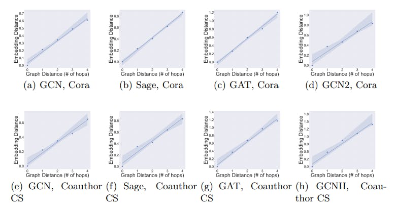
Distance Awareness of the Selected GNNs. We first verify if the selected GNNs preserve (are aware of) graph distances (with a small distortion rate), by evaluating the relation between the graph distances of test vertices to the training set and the embedding distances (Euclidean distance) of vertex representations to the representations of the training set, i.e., the relation between dspd(v, V0) and dEuclidean(M(v),M(V0)). In this experiment, we train the GNN models on the default training set provided in the dataset. We extract vertices within the 5-hop neighbourhood of the training set and group the vertices based on their distances to the training set. 5-hop neighbourhood is chosen because the diameter of most real-life networks is around 5 and it gives a better visual presentation. We then compute the average embedding distance of each group to the training set in the embedding space. Based on Def. 3, if an embedding has low distortion, we should expect to see linear relation with the slope being the scaling factor. As shown in Fig. 3, there exists a strong correlation between the graph distance and the embedding distance. The relation is near linear and the relative orders of distances are mostly preserved within the first few hops. This implies that the distortion α is small with the selected GNNs, i.e., they are distance aware. It also indicates that the premise of the small distortion in our theoretical results can be commonly satisfied in practice.

5.1 Graph Distance and Generalization Performance

Next, we study the relation between graph distance and generalization performance following the same settings as in the previous experiment. We compute the average prediction accuracy in each group of vertices. In Fig. 4, ‘0 hop’ indicates the training set. We observe that the selected GNNs (with low distortion) indeed tend to generalize better on the group of vertices that are closer to the training set, which validates Theorem 2.

We further validate if the distance between different pairs of the training sets and the test group is related to the generalization performance of GNNs in the test group. We randomly sample k = 5 vertices from each class as the training set V0. Then we evaluate the GNN model on the rest of the vertices V\V0. We make k relatively small to enable a larger variance (among different trials) in the distance Dspd(V\V0, V0) (as given in Def. 2) between the training set and the rest of the vertices. We conduct 30 independent trials each selecting a different training set and ranking all the trials in descending order of the mean graph distance between the training set and the rest of the vertices. In Table 1, Group 1 contains the 10 trials with the largest graph distance Dspd(V\V0, V0) and Group 3 includes the 10 trials with the smallest graph distance Dspd(V\V0, V0). The average classification accuracy and the variance (value in the bracket) are computed for each group.

As shown in Table 1, training GNNs on a training set with a smaller graph distance Dspd(V\V0, V0) to the rest of the vertices, does generalize better, which validates our result and further enables us to use these insights for designing and developing new GNNs algorithms.

5.2 Application in Cold Start Problem for Graph Active Learning

Active learning is a type of machine learning where the model is actively involved in the labelling process of the training data. In active learning, the model is initially trained on a small labelled dataset and then used to select the most informative examples from the unlabeled dataset to be labelled next. Unsatisfactory initial set selection can lead to slow learning progress and unfair performance, which is referred to as the cold start problem [11]. Effective resolution of this issue entails an initial set selection that adheres to the following criteria: 1) exclusively leveraging graph structure; 2) achieving robust generalization; and 3) ensuring fairness (with minimal discrepancy in generalization performance) across distinct subgroups. We illustrate how our derived findings can be instrumental in the selection of an effective initial labelled dataset.

Our empirical results show that the selected GNNs are highly distance-aware, meaning that their generalization performance is closely related to the coverage of the training set. To ensure that the model is fair and effective, the initial labelled set should consist of vertices that are in close proximity to the rest of the input graph (in graph distance), as illustrated in Fig. 2. This can be formulated into the following optimization problem:

where k is the given initial set size and Ds(.) is given in Def. 2. Intuitively, Eq.6 aims to select a subset of vertices that exhibit the closest structural similarity (as defined by the graph distance in this case) to the remaining vertices. This problem corresponds to the well-known k-center problem in graph theory [14], which is NP-hard. While finding the optimal solution may be intractable, efficient heuristics exist for tackling Eq. 6. Exploring the best heuristic is beyond the scope of this paper. Instead, for our experiment, we adopt the classic farthest-first traversal algorithm to obtain a solution. We refer to this sample selection procedure as the coverage-based sampling algorithm and provide a detailed description of the method used in the experiment within the supplementary material.

We evaluate the initial set selected by our coverage-based sampling algorithm, comparing it to the existing baselines: (1) R: uniform random sampling [31], and importance sampling with graph properties (2) Degree [15], (3) Centrality, (4) Density and (5) PageRank [5]. We apply each strategy to select an initial dataset of 0.5% of the total data for labelling (training). We evaluate the performance of the learnt model with the rest of the vertices on two metrics: 1) classification accuracy, which reflects the generalization performance, and 2) the maximum discrepancy among structural groups [1, 8], which reflects the fairness. Let Ri denote the mean classification accuracy of the vertex group that is i-hop away from V0. Then, the maximum discrepancy is computed as max{|Ri − Rj ||i, j ∈ 1, ..., r}, where r is the maximum hop number. We use r = 5 to keep consistent with other experiments. The results in Table 2 show that coverage-based sampling achieves a significant improvement in model performance and fairness over the other strategies across different datasets, giving a better kick-start to the active learning process of GNNs.