
In the last two blog posts (here and here), I explained how we can use dbx and asset-bundle to build a CI pipeline. These tools are the basis we need for implementing our MLOps workflow on Databricks.
In this blogpost series we will dive into building an end-to-end MLOps using Databricks and Spark. We will use the Databricks reference architecture as described here. My aim is to break this architecture into smaller components and explain them through a hands-on project.
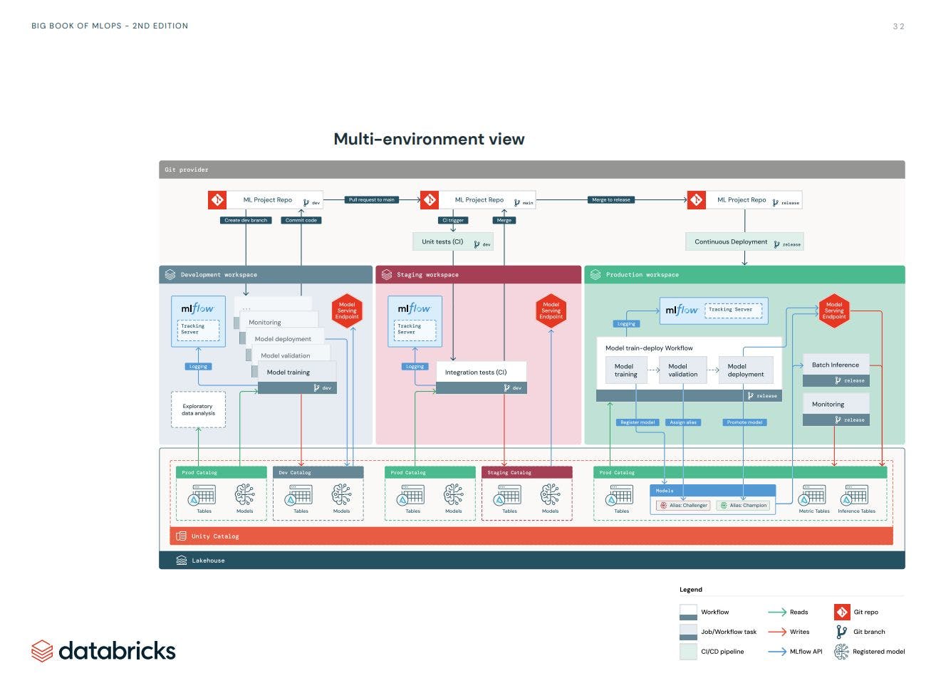
The primary source of this blog series is Databricks documentation. There you can find pretty most of what you read here. However, the reference documentation most useful if you know what you are looking for. If you are new to MLOps, there is a good chance that you don’t how different pieces come together and going through the documentation could be very overwhelming. Here I like to help you to bring these pieces together around a specific use case. I am not going to bore you with detailed explanation of every tools and concepts, but rather direct you to existing resources.
As Databricks keeps evolving sometimes there are more than one way to achieve the same things. One example is Unity Catalog. Databricks keeps integrating and replacing services. So the old way of doing stuff still exists (e.g. model registry) but are no longer the best choice. I try to point out alternatives and provide explanations whenever I think it could help you to avoid confusion!
I divide this series into three parts:
- Data Ingestion and Model Training: We start by setting up the medallion architecture in our Unity Catalog. Then, we go through the various steps of the ML pipeline, including data ingestion, data transformation, feature engineering, model training, and model evaluation. We'll see how to leverage Databricks' Feature Store, Model Registry, and Model Registry to track and version our features, experiments, and models.
- Model Deployment and Monitoring: In this part, we explore how to use Databricks' Feature Store, Model Registry, and Model Serving to deploy our model for batch and online inference. We'll also cover how to log and monitor model and data performance over time using Databricks Lakehouse Monitoring.
- Orchestration: Databricks provides various tools to programmatically automate the management of jobs and workflows, simplifying the development, deployment, and launch of workflows across multiple environments. These tools are fundamentally built around the Databricks REST API, allowing us to manage and control Databricks resources such as clusters, workspaces, workflows, machine learning experiments, and models. In the final part, we use GitLab and the Databricks Asset Bundle to implement a full CI/CD pipeline that manages the complete model lifecycle from development to staging and production.
If you want to refresh your knowledge about higher-level MLops principles I suggests the to have look at these two articles:
- MLOps Principles (ml-ops.org)
- MLOps: Continuous delivery and automation pipelines in machine learning | Cloud Architecture Center | Google Cloud
Ok let’s start with the basics
Databricks
In Databricks everything is built on a Data Lakehouse. This creates a unified system to manage and maintain data and models that are used and built in the MLOps lifecycle. The engine behind the DataOps is Databrick Delta Lake and in particular Databricks Unity Catalog. We will take a short at look at that later. For ModelOps Databricks integrates MLFlow into it Data Lakehouse for operations such as experiment tracking, model registry and model serving. And finally Databricks integrates Git systems for DevOps practices such as CI/CD.

Use case: Movie Recommendation
For the use case, we will work on building a recommender system using the MovieLens dataset. The goal is to suggest new movies to users based on their previous ratings. In this post, we implement collaborative filtering using the Alternating Least Squares (ALS) matrix factorisation method. We use Spark ALS distributed algorithms to train and test the model on our Databricks cluster. We use Spark RegressionEvaluator to evaluate our model. Here we focus on development with Notebooks.
Environment Set-up
Unity Catalog (UC)
The first step to setup the project is to decide how we want to organise our data and AI access. Databricks uses a Hive Metastore (legacy solution) and Unity Catalog - UC (recommended solution) to govern data and AI assets. At the core, they are both centralised metadata management services that store information such as storage locations, table definitions, partition information, and schema details. Unity Data Catalog extends the functionality of the Hive Metastore for better cataloging, discovery, sharing and governance of various assets that are part of the Lakehouse architecture and work seamlessly in the Databricks ecosystem. I recommend to check out the release note and Data, Analytics and AI Governance . Databricks plans to bring all it’s services under the UC and deprecate the legacy services in the future. That’s why in this tutorial we focus on using UC catalog for all the services including Feature Store, Model Registry, Model Serving and etc. Here is the data object hierarchy in Unity Catalog:
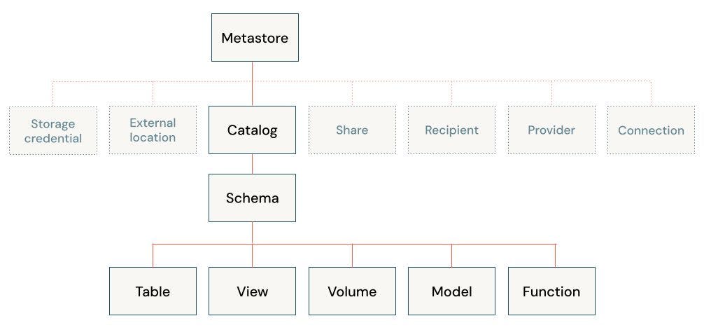
I don’t explain each component here. You can find them in links that I provided earlier. But it is important to understand two things:
-
we can create as many Catalogs as we need. For example it is common to have a separated catalog for development, staging and production assets (requires permission)
-
the unity catalog uses a three-level namespace to address its assets. for example
<catalog>.<schema>.<table>or<catalog>.<schema>.<volume>
Check out this page and make sure your workspace is enabled for UC.
Data Organization
To structure our data on UC, we follow the Medallion Architecture . It is one of the recommended ways to organise your data and is based on data maturity. The architecture typically has three layers, represented as schemas: bronze (raw), silver (structured), and gold (enriched). Depending on your specific use case or team setup, you might have some other layers. For example, you might need to transform you raw dataset in different ways to fit for different use cases, or different segment of your team.
For our use case we keep it simple and specify three schemas as follows:
- raw (bronze): raw data collected from the Movielens data archive. We use the
curlcommand to download the dataset as a.zipfile into thevolumestorage. We also extract the content of the zipped file in the same location. We end up with a collection of.tsvfiles - transformed (silver): we enforce schemas and filter columns for our data tables. This is also where data preprocessing and cleaning takes place.
- feature_store (gold): this schema contains all our aggregated data that can be fed to our ML pipeline.
Create the Catalog and Schemas
To create our catalog and schemas we can either use Databricks UI or by writing SQL commands in a notebook or Databricks SQL editor. Here we use notebooks. let’s assume that you already specific the name of your catalog and schemas in a config.json file.
# create the catalog
spark.sql(f"CREATE CATALOG IF NOT EXISTS {catalog_name}")
spark.sql(f"USE CATALOG  {catalog_name}")

# create the schemas
spark.sql(f"CREATE SCHEMA  IF NOT EXISTS {bronze_layer}")
spark.sql(f"CREATE SCHEMA  IF NOT EXISTS {silver_layer}")
spark.sql(f"CREATE SCHEMA  IF NOT EXISTS {gold_layer}")
spark.sql(f"CREATE SCHEMA  IF NOT EXISTS {output_schema}")

# this is the volume where we download the data from the Movielens archive to
spark.sql(f"CREATE VOLUME {catalog_name}.{bronze_layer}.{volume_name};")
Data Ingestion and Transformation
Bronze Layer
Now that we have setup our data architecture, we can go ahead and get the data into our Databricks workspace. Here we use the bash command curl to download the database directly from the Movielens server. But first, we set the catalog and schema names as environment variables so we can use them in our %sh cells:
import os

database = config["catalog_name"]
boronze_layer = config["bronze_layer_name"]
volume_name = config["ingest_volume_name"]

os.environ["database"] = database
os.environ["bronze_layer"] = bronze_layer
os.environ["volume"] = volume_name
now we can finally get the data, unzip it, and see list its content
%sh
curl  http://files.grouplens.org/datasets/movielens/ml-100k.zip -o /Volumes/$database/$bronze_layer/$volume/ml-100k.zip
unzip /Volumes/$database/$bronze_layer/$volume/ml-100k.zip -d /Volumes/$database/$bronze_layer/$volume/
ls   /Volumes/$database/$bronze_layer/$volume/ml-100k/
Now we have the data as text files.
Silver Layer
The next step is to load and save them as tables with the right schema.
Let’s start with the user-item rating table:
# Define the file path
file_path = f"/Volumes/{database}/{bronze_layer}/{volume_name}/ml-100k/u.data"

#define the schema
df_rating_schema = StructType([
    StructField("user_id", IntegerType(), True),
    StructField("item_id", IntegerType(), True),
    StructField("rating", IntegerType(), True),
    StructField("timestamp", LongType(), True)
])

# Read the data into a DataFrame
df_ratings = spark.read.option("delimiter", "\t") \
                .schema(df_rating_schema) \
                .csv(file_path, header=False) \
                .toDF("user_id", "item_id", "rating", "timestamp")

#convert the timestamp
df_ratings = df_ratings.withColumn("timestamp", from_unixtime("timestamp"))
df_ratings = df_ratings.withColumn("timestamp", to_timestamp("timestamp", "yyyy-MM-dd HH:mm:ss"))

df_ratings.write.format("delta").mode("overwrite").saveAsTable(f"{database}.{silver_layer}.{user_item_table_name}")


display(df_ratings)
and the item-table
# Define the file path
file_path = f"/Volumes/{database}/{bronze_layer}/{volume_name}/ml-100k/u.item"

#define the schema
df_item_schema = StructType([
    StructField("movie_id", IntegerType(), True),
    StructField("movie_title", StringType(), True),
    StructField("release_date", StringType(), True),
    StructField("video_release_date", StringType(), True),
    StructField("IMDb_URL", StringType(), True),
    StructField("unknown", IntegerType(), True),
    StructField("Action", IntegerType(), True),
    StructField("Adventure", IntegerType(), True),
    StructField("Animation", IntegerType(), True),
    StructField("Childrens", IntegerType(), True),
    StructField("Comedy", IntegerType(), True),
    StructField("Crime", IntegerType(), True),
    StructField("Documentary", IntegerType(), True),
    StructField("Drama", IntegerType(), True),
    StructField("Fantasy", IntegerType(), True),
    StructField("FilmNoir", IntegerType(), True),
    StructField("Horror", IntegerType(), True),
    StructField("Musical", IntegerType(), True),
    StructField("Mystery", IntegerType(), True),
    StructField("Romance", IntegerType(), True),
    StructField("SciFi", IntegerType(), True),
    StructField("Thriller", IntegerType(), True),
    StructField("War", IntegerType(), True),
    StructField("Western", IntegerType(), True)
])


# Read the data into a DataFrame
df_item = spark.read.option("delimiter", "|") \
                .schema(df_item_schema)\
               .csv(file_path, header=False) \
               .toDF("movie_id", "movie_title", "release_date", "video_release_date","IMDb_URL",\
                   "unknown","Action","Adventure","Animation", "Childrens", "Comedy", "Crime", "Documentary",\
                    "Drama", "Fantasy", "FilmNoir", "Horror", "Musical", "Mystery", "Romance",\
                    "SciFi", "Thriller", "War", "Western")

df_item = df_item.withColumn("release_date", to_timestamp("release_date", "d-MMM-yyyy"))
df_item.write.format("delta").mode("overwrite").option("overwriteSchema", "true").saveAsTable(f"{database}.{silver_layer}.{items_table_name}")

display(df_item)
we repeat this process to create the genre and the occupation tables
Gold Layer - Feature Store (FS)
Next, we are in the last layer of data transformation. The result of this layer can be fed directly to our model training pipeline. We store the result of this layer as feature tables using Databricks Feature Store API. In short, a feature store is a data “management” layer that act as an interface between your data and model. The “interface” aspect is to suggest that your data in the feature store is directly connected to the models that use that data, and also to the code that created those features. Feature stores help us with feature Discovery (finding, sharing and reusing the features), Lineage (tracking how the feature is generated and being used), Skew ( reproducing the necessary input data and data transformations logic for training and inference). If you are not familiar with the feature store, I suggest to check out The Comprehensive Guide to Feature Stores | Databricks.
The implementation of a feature store in Databricks depends on if your workspace is enabled for Unity Catalog or not. In workspaces that are enabled for Unity Catalog, any Delta table serves as a feature table, and Unity Catalog acts as a feature store — no separate step is needed to register a table as a feature table. Workspaces that are not enabled for Unity Catalog have access to the Workspace Feature Store.
Databricks offers two ways to create, store and manage features. For workspaces that are enabled for Unity Catalog we can use Databricks Feature Engineering in Unity Catalog. In this case, the Unity Catalog serve as a feature store and any Delta table serves as a feature table. That means we can use an existing Delta table in Unity Catalog as a feature table. For workspaces that are not enabled for Unity Catalog we would use the Databricks Workspace Feature Store legacy solution. We will go with the first solution, as the latter will become obsolete sooner or later.
First we select/use the catalog and schema
spark.sql(f"USE CATALOG {database}")
spark.sql(f"USE SCHEMA {gold_layer}")
Install the databricks-feature-engineering package:
%pip install databricks-feature-engineering

dbutils.library.restartPython()
Create a FeatureEngineeringClient instance:
from databricks.feature_engineering import FeatureEngineeringClient

fe = FeatureEngineeringClient()
Now we can read, transform and save the tables as feature table. Two important notes about the feature tables:
- They should not include your target/label column but only features that will be used to build the model
- Each feature table needs to have at least one
primary key. Databricks use them to create the final training set by joining the feature table with the data frame that include the target/label column.
We start with the user-item-ranking table
import pyspark.sql.functions as F


df_ratings = spark.table(f"{catalog_name}.{silver_layer}.{user_item_table_name}")

# --- create two new features rating_date_month and rating_date_dayofmonth
df_ratings_transformed = df_ratings.withColumnRenamed("timestamp", "rating_date")
df_ratings_transformed  = df_ratings_transformed.withColumn("rating_date_month",F.month("rating_date")).withColumn("rating_date_dayofmonth",F.dayofmonth("rating_date"))

# --- drop the target column
df_ratings_transformed = df_ratings_transformed.drop("rating_date","rating")

# --- feature table name
table_name = f"{catalog_name}.{gold_layer}.{config['ft_user_item_name']}"

# --- create and write the feature store
if spark.catalog.tableExists(table_name):
    #to update the table
    fe.write_table(
        name=table_name,
        df=df_ratings_transformed,
    )
else:
    fe.create_table(
        name=table_name,
        primary_keys=config['ft_user_item_pk'],
        df=df_ratings_transformed,
        schema=df_ratings_transformed.schema,
        description=config['ft_user_item_des']
    )
and user table:
df_users = spark.table(f"{catalog_name}.{silver_layer}.{users_table_name}")

#--- create a categorical variable for the age variable

from pyspark.sql.functions import udf

@udf(returnType=IntegerType())
def categorize_age(age):
    if age >= 0 and age <= 15:
        return 1
    elif age > 15 and age <= 20:
        return 2
    elif age > 20 and age <= 30:
        return 3
    elif age > 30 and age <= 40:
        return 4
    elif age > 40 and age <= 50:
        return 5
    elif age > 50 and age <= 60:
        return 6
    elif age > 60 and age <= 70:
        return 7
    elif age > 70 and age <= 80:
        return 8
    else:
        return None

df_users_transformed = df_users.withColumn("age_category", categorize_age("age"))

table_name = f"{catalog_name}.{gold_layer}.{config['ft_users_name']}"

if spark.catalog.tableExists(table_name):
    #to update the table
    fe.write_table(
        name=table_name,
        df=df_users_transformed,
    )
else:
    fe.create_table(
        name=table_name,
        primary_keys=config['ft_users_pk'],
        df=df_users_transformed,
        schema=df_users_transformed.schema,
        description=config['ft_users_des']
    )
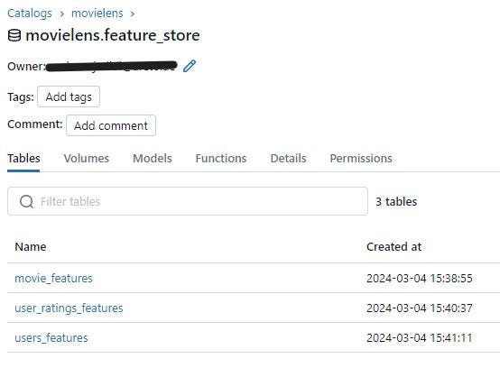
we do the same for the movie tables. Now if you go to your catalog, you will find all your feature tables:
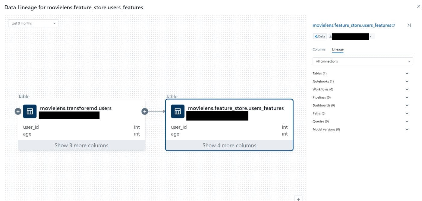
Now you can click of any of the table and check their lineage. Here is how it looks like for the users_features table. here we can see that this table is instantiated from the users table. We can also find the link to the notebook that create this table.
Model Training, Experiment Tracking and Model Registry
Now that we have the features ready we can use them train our model. As we train our models we like to log the model artifacts, parameters and performances metrics. We use Hyperopt for parameter tuning while keeping track of the performance model under each set of parameters. Finally, we find the best model and register it to our UC to later load it for our inference pipeline. Let’s see how it all work.
Creating Dataset
The first step is to create the training set by joining the feature table with the Dataframe that contains the target column (i.e. ratings). To do this we can use FeatureLookup . The FeatureLookup specifies which features to use from the table, and also defines the keys to use to join the feature table to the label data passed to create_training_set. The following diagram shows how it works (more here).
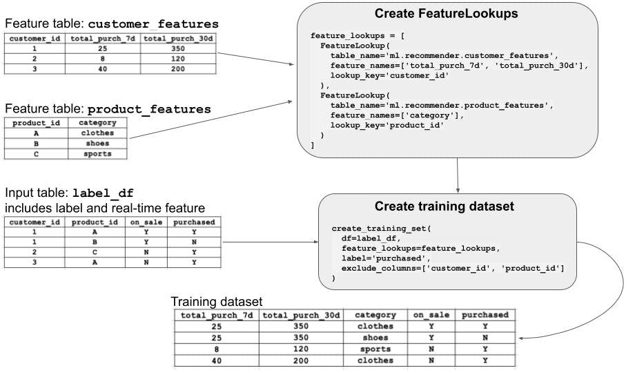
Since we want to use the ALS algorithm for building a Collaborative Filtering recommender system, we only need the user-item feature table. After creating the training set, we split it to training and test set for model evaluation.
#create_training_set.py

import json
from databricks.feature_engineering import FeatureEngineeringClient, FeatureLookup

#--- read the config file
with open('config.json') as config_file:
    config = json.load(config_file)

catalog_name = config["catalog_name"]
gold_layer = config["gold_layer_name"]
silver_layer = config["silver_layer_name"]
user_item_table_name = config["user_item_table_name"]
ft_user_item_name = config["ft_user_item_name"]
model_name = config["model_name"]

#inite the API
fe = FeatureEngineeringClient()

def split_data():
    SEED = 4

    df_ratings = spark.table(f"{catalog_name}.{silver_layer}.{user_item_table_name}")

    table_name = f"{catalog_name}.{gold_layer}.{ft_user_item_name}"
    lookup_key = config["ft_user_item_pk"]
    label = config["label_col"]
    model_feature_lookups = [FeatureLookup(table_name=table_name, lookup_key=lookup_key)]

    # fe.create_training_set looks up features in model_feature_lookups that match the primary key from df_ratings
    fe_data = fe.create_training_set(df=df_ratings, feature_lookups=model_feature_lookups, label=label)
    df_data = fe_data.load_df()
    df_data = df_data.na.drop()

    # ----  Split data into training and test sets
    (df_train, df_test) = df_data.randomSplit([0.75,0.25],SEED)
    print(f'full dataset: {df_data.count()}' ,f'Training: {df_train.count()}', f'test: {df_test.count()}\n')
    return (fe_data, df_data, df_train, df_test)
Experiment Tracking with MLflow
Before diving into the practical part it is important to understand the key concept behind the model tracking and registry. So let’s spend some time on it before we go to the hands-on part. I would still keep it short and point to other resources with comprehensive explanation. Feel free to jump to the hands-on part if you already know the basics.
Experiment tracking
Experiment tracking is a fundamental aspect of the machine learning lifecycle. Within your ML lifecycle, you may want to use different libraries to train different models, with different hyperparameters. Specially as the project get bigger and more complex, it becomes more important to keep track of different experiments that you run. This include keeping track of the models, results, parameters, code, data schema, data samples, and supplementary artifacts such a feature weight, coefficient importance plots, etc.
In Databricks we can use MLflow for experiment tracking. MLflow offers a library and environment agnostic API to record ML Experiments. Experiments are the primary unit of organization in MLflow. Each experiment consist of a group of related Runs. An MLflow run corresponds to a single execution of model code. When you run an experiment or train a model, it creates a run.
There are two types of experiment runs in Databricks (read more here):
- Workspace experiment: we can create a workspace experiment that can log the run of any experiment in your notebook by using the experiment ID or name.
- Notebook experiment*: experiment is assigned to a specific notebook. By default Databricks creates an experiment with the name and id of the corresponding notebook when we use the MLflow API to log a run. We use this option!
💡 we have to set the experiment name explicitly using the full path when we run a notebook using Databricks jobs. more in that in part 3!
To read more about MLflow experiment tracking check out the official tutorial and Databricks example notebooks.
Model Registry
Databricks offer various solutions to register a model and these solutions seems to changer over time. Databricks currently offer two ways to register the model:
-
Workspace Model Registry (legacy): This is the old way of how Databricks handle the model registry. In this case, the model is stored on the Workspace DBFS path. This entails we don’t have a central model registry that can be accessed by different teams and environments. This could create some complication when we want to have separate environments for developing , testing and deploying our model. To deal with such scenarios, one option is to have dedicated workspace to store models, feature tables, and experiments as central space to manage all the models.
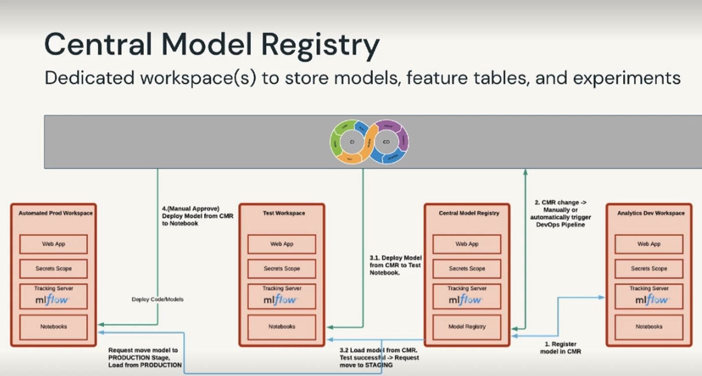
- Unity Catalog Model Registry: store model to the Unity Catalog-configured storage location. Here we can benefit from the advanced governance capabilities to share the models across the workspace and environments.
Here is the comparison between the two solutions: Manage model lifecycle in Unity Catalog - Azure Databricks | Microsoft Learn
- Model registry with Feature Store/Engineering: We can also log and register models with
FeatureEngineeringClient.log_model(for Feature Engineering in Unity Catalog) orFeatureStoreClient.log_model(for Workspace Feature Store). When we train a model in this way it automatically tracks the features, tables and function that are used to train the model. When we're using the model to make predictions, it can grab those feature values from the Feature Store. In batch mode, it fetches values from the offline store and mixes them with new data before making predictions. In real-time inference, values are obtained from the online store.
Hands-on
now let’ see how it all works in practice!
To be able use models in Unity Catalog we need Databricks Runtime 13.2 LTS and above, and the latest version of MLflow Python client:
%pip install --upgrade "mlflow-skinny[databricks]"
dbutils.library.restartPython()
We also need to tell MLflow that we want to use Unity Catalog to store our models
mlflow.set_registry_uri("databricks-uc")
we can set the experiment name as follows. But for now we skip setting the experiment explicitly and let it adapt the notebook name.
#mlflow.set_experiment(config["experiment_name"])
now we can go ahead and train our model
from pyspark.mllib.recommendation import ALS, MatrixFactorizationModel, Rating
from pyspark.ml.evaluation import RegressionEvaluator

from create_training_set import split_data


COL_PRED = 'prediction'
COL_USER = config['user_col']
COL_ITEM = config['item_col']
COL_LABEL = config['label_col']

# -- define hyperparamteres
RANK = 2
SEED = 4
MAX_ITER = 20
REG_PARAM = 0.01

# --- split train and validation sets
fe_full_data, df_full_data, df_train, df_test = split_data()

#activate the experiment tracking by setting the run name
with mlflow.start_run(run_name="als-model") as run:
		 # --- Instantiate the model and and set the parameters
        als = ALS()
        als.setMaxIter(MAX_ITER)\
        .setSeed(SEED)\
        .setRegParam(REG_PARAM)\
        .setUserCol(COL_USER)\
        .setItemCol(COL_ITEM)\
        .setRatingCol(COL_LABEL)\
        .setRank(RANK)

		# --- log the model parameters
        mlflow.log_param("MAX_ITER", MAX_ITER)
        mlflow.log_param("RANK", RANK)
        mlflow.log_param("REG_PARAM", REG_PARAM)

        # --- fit the model with these parameters.
        model = als.fit(df_train)
        #--- drop predictions where users and products from the test set didn't make it into the training set. in this case, the prediction is NaN
        model.setColdStartStrategy('drop')

		# --- Run the model to create a prediction. Predict against the validation_df.
		predictions = model.transform(df_sample_validation)
        # log the prediction table as an artifact
        predictions.toPandas().to_csv('../data/predictions.csv', index=False)
        mlflow.log_artifact("../data/predictions.csv")
        #or as a table in UC
        # --- save the prediction results to the schema of our catalog.
        predictions.write.mode("overwrite").saveAsTable(f"{catalog_name}.{output_schema}.predictions")


		# --- infer and log the model with signature and input example
        signature = infer_signature(model_input = df_train, model_output = predictions.select(COL_LABEL))
		input_example = df_sample_training.limit(3)

		# --- log the model
		# we can skip the `signature` and let it automatically inferred from sample input and prediction data
        mlflow.spark.log_model(model, model_name,
                               signature=signature,
							   sample_input=input_example
                               conda_env=mlflow.spark.get_default_conda_env(),
                               registered_model_name = f"{catalog_name}.{model_schema}.{model_name}")


		# --- log different evaluation metrics
        evaluator = RegressionEvaluator(predictionCol=COL_PRED, labelCol=COL_LABEL)
		rmse = evaluator.setMetricName("rmse").evaluate(predictions)
        r2 = evaluator.setMetricName("r2").evaluate(predictions)
        mse = evaluator.setMetricName("mse").evaluate(predictions)
        mae = evaluator.setMetricName("mae").evaluate(predictions)

        mlflow.log_metric("rmse", rmse)
        mlflow.log_metric("r2", r2)
        mlflow.log_metric("mse", mse)
        mlflow.log_metric("mae", mae)
Everything should be pretty self explanatory, maybe except signature and conda_env arguments in the model logging. These parameters are used to ensure the integrity, reproducibility of the model during deployment and serving.
- signature is there is to make sure your model’s input and output in the inference stage are in the correct format and type. For example, if your model is trained using three variables
[a,b,c], but the input toload_model.predict(input_df)receives only two variables, the mlflow raise an Exception from schema enforcement telling you which variables are missing. More on signature enforcement here. Model in UC must have a model signature. - conda_env: this is to make sure your deployment environment include all the model dependencies including all libraries and packages. If you don’t specify this parameter, MLflow infer and log the model dependencies automatically. still I find it helpful to understand know what happens in the background. check our Managing Dependencies in MLflow Models for more.
Every time your run this code, a new version of the model would be registered in your UC! After running the code you can navigate to your Experiment window and find:
-
an experiment with the name of your notebook ( 5_ALS_training ) → screenshot 1 in figure below
-
click on the experiment and you should see all the runs that are associated with this experiment. (als-model) → ****screenshot 2
-
next click on the run to see all the model parameters, metrics, and artifacts. Navigate to the Artifact tab to see model schema, sample input, etc.

now if you click on the Registered models it will direct you the default schema (set by config[“model_schema”]) of your catalog. As you can see in the figure below, the model version is 3. That means we run the model training 3 times.
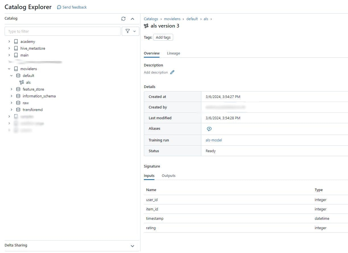
Hyperparameter Turning (Nested Runs)
Here we look into the hyperparameter tuning using HyperOpt to find the best the values for REG_PARAMS and RANK .
MLflow offers a useful tool to organize runs in a tree structure format. One of the common use cases for this tool is hyperparameter tuning. Every runs of model with new hyperparameters will be logged under a parent run. This allow us to compare the models to find the best hyperparameters. Another use case would be training a neural network and checkpoint results after n epochs with all the associated artifacts and metrics.
For that we have to make some changes to our code. Let’s specify our search space first.
from hyperopt import fmin, tpe, hp, SparkTrials, STATUS_OK

REG_PARAMS = hp.uniform('REG_PARAM', 0.001, 0.1)
RANKS = hp.quniform("RANK", 4, 12,1)

search_space = {"REG_PARAM": REG_PARAMS,
                "RANK": RANKS,
                }
Then we need to define a objective function to minimize. That is the function should return a loss metric (for which lower is better), so in case you want to work with accuracy metrics such as f1 score, the function should the negative value, e.g., f1_score
def train_with_hyperopt(params):
  reg_param = params['REG_PARAM']
  rank = params['RANK']

  model, predictions, loss, run_id = train_als(reg_param, rank)
  return {'loss': loss, 'status': STATUS_OK}
as you can see we call the train_als function which is basically our model training code as a function but this time we set the nested=True parameter to true. We also leave out the manual logging and use autolog instead.
mlflow.autolog(exclusive=False, log_models=False)

def train_als(REG_PARAM, RANK):
    (df_sample_training, df_sample_validation) = df_train.randomSplit([0.75, 0.25],SEED)
    # Specify "nested=True" since this single model will be logged as a child run of Hyperopt's run.
    # --- starting the MLflow run
    with mlflow.start_run(nested=True) as run:
        # --- Instantiate the model and set the parameters
		als = ALS()
        als.setMaxIter(MAX_ITER)\
        .setSeed(SEED)\
        .setRegParam(REG_PARAM)\
        .setUserCol(COL_USER)\
        .setItemCol(COL_ITEM)\
        .setRatingCol(COL_LABEL)\
        .setRank(RANK)
				# --- model trainig and evaluation
        model = als.fit(df_full_data)
        model.setColdStartStrategy('drop')
        predictions = model.transform(df_sample_validation)
	    evaluator = RegressionEvaluator(predictionCol=COL_PRED, labelCol=COL_LABEL)
        rmse = evaluator.setMetricName("rmse").evaluate(predictions)
		return rmse
finally we tune the model using the Hyperopt fmin() optimization function. The function receives an objective function, hyperparameter search space, and a search algorithms to find the best combination of values in a “smart” way instead of grid search. You can read more about other fmin() arguments here.
mlflow.autolog(log_models=False)

with mlflow.start_run(run_name="ALS_Hyperopt"):
    best_params = fmin(fn=train_with_hyperopt,
                    space=search_space,
                    algo=tpe.suggest,
                    max_evals=8,
                    )


print(best_params)

#{'RANK': 12.0, 'REG_PARAM': 0.014978776269755367}
if you want to use Sklearn: Here we use Hyperopt with distributed training algorithms (ALS from Spark mllib library). However, when we use algorithms that are not themselves distributed (e.g. sklearn), we can use SparkTrials for parallel training of our model. In this case, the function call would look like the following. More on this here.
# Set parallelism (should be order of magnitude smaller than max_evals)
spark_trials = SparkTrials(parallelism=2)

with mlflow.start_run(run_name="Hyperopt"):
    argmin = fmin(fn=objective,
                  space=search_space,
                  algo=tpe.suggest,
                  max_evals=8,
                  trials=spark_trials)
Model Evaluation
The purpose of model evaluation is to measure the quality of the model on a hold-out test set. In practice, we use the result of this test to check if a newly trained model (refers to candidate or challenger model) can outperform our existing deployed model in the production (refers to champion model). If it does, we should update the production model with the new model. Since we don’t have a production model in this example we skip the comparison part. But we come back to it in the next blog post.
now we can use the optimized parameters to retrain our model and test it on our hold-out set.
with mlflow.start_run(run_name="ALS_candidate_model") as run:

        als = ALS()
        als.setMaxIter(MAX_ITER)\
        .setSeed(SEED)\
        .setRegParam(best_params["REG_PARAM"])\
        .setUserCol(COL_USER)\
        .setItemCol(COL_ITEM)\
        .setRatingCol(COL_LABEL)\
        .setRank(best_params["RANK"])

        mlflow.log_param("MAX_ITER", MAX_ITER)
        mlflow.log_param("RANK", best_params["RANK"])
        mlflow.log_param("REG_PARAM", best_params["REG_PARAM"])

        model = als.fit(df_train)
        model.setColdStartStrategy('drop')
        predictions = model.transform(df_test)
        # --- save the prediction results to the default schema of our catalog.
        predictions.write.mode("overwrite").saveAsTable(f"{catalog_name}.{model_schema}.predictions")

        evaluator = RegressionEvaluator(predictionCol=COL_PRED, labelCol=COL_LABEL)
        rmse_test = evaluator.setMetricName("rmse").evaluate(predictions)
        mlflow.log_metric('rmse', rmse_test)
如有侵权请联系:admin#unsafe.sh